41 align data labels excel chart

Can't edit charts - all options greyed out - Microsoft Tech Community Hi - I've recently been upgraded to Office 365. I've got a regular reporting spreadsheet, with charts that need updating. However, I can't edit any of the charts! I can't right click anywhere on the sheets containing the charts, and all the options on the 'Chart Design' and 'Format' ribbon tabs are greyed out. How to Change the Y Axis in Excel - Alphr Click the dropdown next to "Display Units," then make your selection such as "millions" or "hundreds." To label the displayed units, go to the "Axis Options -> Display units" section. Add a...

DataLabel.HorizontalAlignment property (Excel) | Microsoft Docs In this article. Returns or sets a Variant value that represents the horizontal alignment for the specified object.. Syntax. expression.HorizontalAlignment. expression A variable that represents a DataLabel object.. Remarks. The value of this property can be set to one of the XlHAlign constants.. Some of these constants may not be available to you, depending on the language support (U.S ...

Align data labels excel chart

Excel Waterfall Chart: How to Create One That Doesn't Suck If your data has a different number of categories, you have to modify the template, which again requires additional work. Ideally, you would create a waterfall chart the same way as any other Excel chart: (1) click inside the data table, (2) click in the ribbon on the chart you want to insert. ... in Excel 2016 Custom Excel number format - Ablebits A usual way to change alignment in Excel is using the Alignment tab on the ribbon. However, you can "hardcode" cell alignment in a custom number format if needed. ... Is it possible to display a percentage value without the percentage sign using custom number formatting? I want the chart labels for each data point to be displayed without ... Clustered Column and Line Combination Chart - Peltier Tech Excel's column and bar charts use two parameters, Gap Width and Overlap, to control how columns and bars are distributed within their categories. Gap Width is the space between bars in adjacent categories, given as a percentage of the width of a column in the chart. The default is 219%, which means the gap is 2.19 times the width of a column.

Align data labels excel chart. Custom Chart Data Labels In Excel With Formulas Select the chart label you want to change. In the formula-bar hit = (equals), select the cell reference containing your chart label's data. In this case, the first label is in cell E2. Finally, repeat for all your chart laebls. If you are looking for a way to add custom data labels on your Excel chart, then this blog post is perfect for you. How to align graph and the access in Excel - Stack Overflow 1. You can get better alignment between the tics and the data points when using the Line graphs. Scatter plots are designed to be at the measure locations. So change to line graphs. Share. answered Jun 10 at 4:03. Citycreek. How to Change the X-Axis in Excel - Alphr Open the Excel file with the chart you want to adjust. Right-click the X-axis in the chart you want to change. That will allow you to edit the X-axis specifically. Then, click on Select Data. Next ... Formatting Long Labels in Excel - PolicyViz In the ensuing menu, select the Right option in the Alignment drop-down menu. Now, ideally, we'd be able to align the text to the left and everything would be nicely aligned along the left edge, but it aligns to the left within each label, so it doesn't look great, as you can see in the first image below.

Plot Multiple Data Sets on the Same Chart in Excel After insertion, select the rows and columns by dragging the cursor. Step 2: Now click on Insert Tab from the top of the Excel window and then select Insert Line or Area Chart. From the pop-down menu select the first "2-D Line". From the above chart we can observe that the second data line is almost invisible because of scaling. How to Create and Customize a Treemap Chart in Microsoft Excel Either right-click the chart and pick "Format Chart Area" or double-click the chart to open the sidebar. On Windows, you'll see two handy buttons on the right of your chart when you select it. With these, you can add, remove, and reposition Chart Elements. And you can pick a style or color scheme with the Chart Styles button. DataLabel.VerticalAlignment property (Excel) | Microsoft Docs Syntax Remarks Returns or sets a Variant value that represents the vertical alignment of the specified object. Syntax expression. VerticalAlignment expression A variable that represents a DataLabel object. Remarks The value of this property can be set to one of the XlVAlign constants. Support and feedback How to Print Labels from Excel - Lifewire To label legends in Excel, select a blank area of the chart. In the upper-right, select the Plus ( +) > check the Legend checkbox. Then, select the cell containing the legend and enter a new name. How do I label a series in Excel? To label a series in Excel, right-click the chart with data series > Select Data.

Questions from Tableau Training: Can I Move Mark Labels? Option 1: Label Button Alignment. In the below example, a bar chart is labeled at the rightmost edge of each bar. Navigating to the Label button reveals that Tableau has defaulted the alignment to automatic. However, by clicking the drop-down menu, we have the option to choose our mark alignment. Pivot chart X axis labels not aligned to the ... - Excel Help Forum 3) Find the "Series Overlap" setting and change it to "full overlap" or "+100%" or whatever the equivalent is in your version of Excel. I will see if someone more familiar with the O365 UI can provide more details on where and how to find these options. Register To Reply 08-12-2021, 02:19 PM #5 Jigneshbharati Registered User Join Date 12-02-2020 Make Excel charts primary and secondary axis the same scale In the first cell create a MIN function that looks at ALL the original data points and finds the smallest number. In the last cell do the same but this time a MAX to find the biggest number out of all the data points. In E8 and E34 just equals to the adjacent cells. You now know what the scale needs to be. Insert the new series into the chart Two-Level Axis Labels (Microsoft Excel) - ExcelTips (ribbon) Place your row labels into column A, beginning at cell A3. Place your data into the table, beginning at cell B3. With your table completed, you are ready to create the chart. Just select your data table, including all the headings in the first two rows, then create your table.

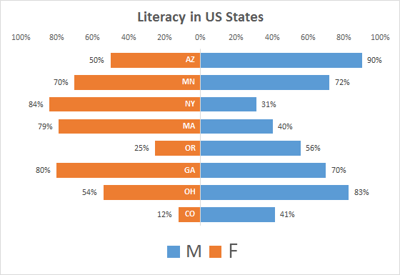
Solution - Challenge 19 – Make Comparative Horizontal Bar Graph | `E for Excel | Excel, VBA ...

How to Add Axis Titles in a Microsoft Excel Chart Select your chart and then head to the Chart Design tab that displays. Click the Add Chart Element drop-down arrow and move your cursor to Axis Titles. In the pop-out menu, select "Primary Horizontal," "Primary Vertical," or both. If you're using Excel on Windows, you can also use the Chart Elements icon on the right of the chart.

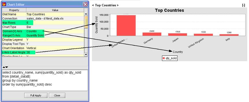
Dashboard using Excel : Create Bar Chart | InfoCaptor Dashboard

How To Tally in Excel by Converting a Bar Graph to a Tally Graph Once you've inputted your data, you can create a tally graph in Excel by converting a bar chart. First, select the 5-Mark and 1-Mark columns, including the 5-Mark and 1-Mark column labels. Then, go to the " Insert" tab in your toolbar and locate the "Charts" section. This section contains a collection of chart icons.

Add Axis Label Excel - Best Label Ideas 2019

Controlling Chart Gridlines (Microsoft Excel) In the Current Selection group, use the drop-down list to choose the gridlines you want to control. Click the Format Selection tool, also within the Current Selection group. Excel displays a Format task pane at the right side of the program window. Use the controls in the task pane to make changes to the gridlines, as desired. Close the task pane.

Enable or Disable Excel Data Labels at the click of a button - How To - PakAccountants.com

Excel Pivot Table Filter and Label Formatting - Microsoft Tech Community Images of 2 separate workbooks, each with a data table, pivot table and pivot chart, the one on the right created by copy & paste of the one on the left. The one on the right changed: X axis labels on the pivot chart don't have the multi-level option. Also, unlike the original on the left, there is now a filter button for the chart.

Horizontal Axis- dates vs text, reverse order, show all labels • Online-Excel-Training ...

Using VBA to Loop Through and Automatically Position Data Labels ... Set mychart = ActiveSheet.ChartObjects ("Chart 4") With mychart.Chart.SeriesCollection (1) Dim myvalues myvalues = .Values Dim i As Long For i = LBound (myvalues) To UBound (myvalues) If .Points (i).HasDataLabel And myvalues (i) < 0 And myvalues (i) > -40 Then Selection.Position = xlLabelPositionOutsideEnd Selection.Top = 146.623 Else

Excel Charts: Positive/Negative Axis Labels on a Bar Chart

Tree Maps Data Labels and Tables Formatting/Sorting Errors after ... Tree Maps Data Labels and Tables Formatting/Sorting Errors after Windows 11. My Tree Map in Excel and Powerpoint after the Windows 11 update does not order my tables from smallest/largest value correctly, nor allow me to right-align my data labels, nor does it spell out the data label name.

Microsoft Tips with Temo!: How to Add Data Labels to an Excel 2010 Chart

5 New Charts to Visually Display Data in Excel 2019 - dummies Select the data and labels and then click Insert → Maps → Filled Map. Wait a few seconds for the map to load. Resize and format as desired. For example, you could apply one of the chart styles from the Chart Tools Design tab. To add data labels to the chart, choose Chart Tools Design → Add Chart Element → Data Labels → Show.

Excel Vba Legend Fill Color - excel vba position chart legend move and align titles fill pattern ...

Best Types of Charts in Excel for Data Analysis ... - Optimize Smart To add a chart to an Excel spreadsheet, follow the steps below: Step-1: Open MS Excel and navigate to the spreadsheet, which contains the data table you want to use for creating a chart. Step-2: Select data for the chart: Step-3: Click on the 'Insert' tab: Step-4: Click on the 'Recommended Charts' button:

Share :