42 excel data labels from third column

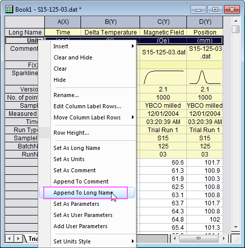
VLOOKUP Hack #4: Column Labels - Excel University This MATCH function would return 2 since the Amount label is in the 2nd table column. So, replacing the 2 in our original formula with the MATCH function would look like this: =VLOOKUP (B5, Table1, MATCH (C4,Table1 [#Headers],0), 0) This technique allows us to reference the column labels instead of the position number. But, Jeff, hang on. Change the format of data labels in a chart To get there, after adding your data labels, select the data label to format, and then click Chart Elements > Data Labels > More Options. To go to the appropriate area, click one of the four icons ( Fill & Line, Effects, Size & Properties ( Layout & Properties in Outlook or Word), or Label Options) shown here.

How to Print Labels from Excel Using Database Connections Open label design software. Click on Data Sources, and then click Create/Edit Query. Select Excel and name your database. Browse and attach your database file. Save your query so it can be used again in the future. Select the necessary fields (columns) that you would like to use on your label template. 😊.

Excel data labels from third column

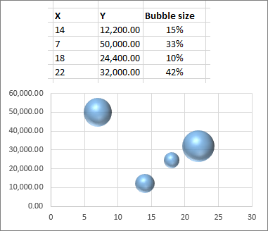
Add Custom Labels to x-y Scatter plot in Excel Step 1: Select the Data, INSERT -> Recommended Charts -> Scatter chart (3 rd chart will be scatter chart) Let the plotted scatter chart be. Step 2: Click the + symbol and add data labels by clicking it as shown below. Step 3: Now we need to add the flavor names to the label. Now right click on the label and click format data labels. How to add data labels from different column in an Excel chart? This method will guide you to manually add a data label from a cell of different column at a time in an Excel chart. 1. Right click the data series in the chart, and select Add Data Labels > Add Data Labels from the context menu to add data labels. 2. How to Create Mailing Labels in Word from an Excel List Step Two: Set Up Labels in Word. Open up a blank Word document. Next, head over to the "Mailings" tab and select "Start Mail Merge.". In the drop-down menu that appears, select "Labels.". The "Label Options" window will appear. Here, you can select your label brand and product number. Once finished, click "OK.".

Excel data labels from third column. Add or remove data labels in a chart - support.microsoft.com Right-click the data series or data label to display more data for, and then click Format Data Labels. Click Label Options and under Label Contains, select the Values From Cells checkbox. When the Data Label Range dialog box appears, go back to the spreadsheet and select the range for which you want the cell values to display as data labels. How to rotate axis labels in chart in Excel? 1. Go to the chart and right click its axis labels you will rotate, and select the Format Axis from the context menu. 2. In the Format Axis pane in the right, click the Size & Properties button, click the Text direction box, and specify one direction from the drop down list. See screen shot below: peltiertech.com › excel-column-Excel Column Chart with Primary and Secondary Axes - Peltier ... Oct 28, 2013 · The second chart shows the plotted data for the X axis (column B) and data for the the two secondary series (blank and secondary, in columns E & F). I’ve added data labels above the bars with the series names, so you can see where the zero-height Blank bars are. The blanks in the first chart align with the bars in the second, and vice versa. Adding rich data labels to charts in Excel 2013 - Microsoft 365 Blog Putting a data label into a shape can add another type of visual emphasis. To add a data label in a shape, select the data point of interest, then right-click it to pull up the context menu. Click Add Data Label, then click Add Data Callout . The result is that your data label will appear in a graphical callout.

Apply Custom Data Labels to Charted Points - Peltier Tech Click once on a label to select the series of labels. Click again on a label to select just that specific label. Double click on the label to highlight the text of the label, or just click once to insert the cursor into the existing text. Type the text you want to display in the label, and press the Enter key. Create a multi-level category chart in Excel - ExtendOffice 1.3) In the third column, type in each data for the subcategories. 2. Select the data range, click Insert > Insert Column or Bar Chart > Clustered Bar. 3. Drag the chart border to enlarge the chart area. See the below demo. 4. Right click the bar and select Format Data Series from the right-clicking menu to open the Format Data Series pane. stackoverflow.com › questions › 55735003Excel Pivot Table with multiple columns of data and each data ... Apr 17, 2019 · This will produce a Pivot Table with 3 rows. The first row will read Column Labels with a filter dropdown. The second row will read all the possible values of the column. The third row will be the count of each value in the above column. Repeat the process in the next available blank cell for the next category, which will produce something like ... How to Use Cell Values for Excel Chart Labels - How-To Geek Select the chart, choose the "Chart Elements" option, click the "Data Labels" arrow, and then "More Options." Uncheck the "Value" box and check the "Value From Cells" box. Select cells C2:C6 to use for the data label range and then click the "OK" button. The values from these cells are now used for the chart data labels.

Excel VBA - Add Data Labels from Table body range - Stack Overflow This is code that I use for data labels from a range. Have found this on stackoverflow a while back: Sub DataLables Dim ws as worksheet, DataLR As Series, pts As Points, pt As Point, rngLabels As Range, IDi As Integer, ChtObj As ChartObject Set ws = ActiveWorkbook.ActiveSheet With ws Set ChtObj = .ChartObjects("ChatName") Set rngLabels = .Range("A5:A39") Set DataLR = ChtObj.Chart ... How to Create Labels in Word from an Excel Spreadsheet Select Browse in the pane on the right. Choose a folder to save your spreadsheet in, enter a name for your spreadsheet in the File name field, and select Save at the bottom of the window. Close the Excel window. Your Excel spreadsheet is now ready. 2. Configure Labels in Word. Mac Excel 2008 - How to add Data Labels for Scatter Plot coming from ... In Excel 2008, to select X axis for the labels: go to 'Formatting palette' navigate to 'Chart Option' Under 'Other options' select "category name' in Labels. A AsherS New Member Joined Feb 9, 2012 Messages 9 Jul 30, 2014 #3 Cyrilbrd, this does not add a label from another column. This only displays the X-value and does not solve the issue. cyrilbrd › articles › how-to-export-dataHow to Export Data From Excel to Make Labels - Techwalla Mar 11, 2019 · At this point, take the time to locate the list you named earlier and then click the Select Data Source box. You are presented with a window in which you confirm the specific data source you are using. After clicking the Show all box, select the MS Excel Worksheets via DD option in the Open data source box before pressing OK.

Enable or Disable Excel Data Labels at the click of a button - How To - PakAccountants.com

Data labels not displayed correctly - Excel Help Forum The data label is a date value that selects values from the date column. The Primary axis is categorized based on 2 values. The secondary axis is Month. The data labels are displayed accurately as per the month except the 3 labels. The first series is the difference between F and E.The second series is the difference between the J and K column.

How to edit the label of a chart in Excel? - Stack Overflow

How to compare two columns and return values from the third column in ... The entire Column C items in Sheet 2 to be compared with first row item in Column A and if any corresponding values/data are there in Column A, then Column B to be populated with data corresponding to the row item in Column D. Column C will have a single word. Column D may or may not have data in it. Column A will have more text.

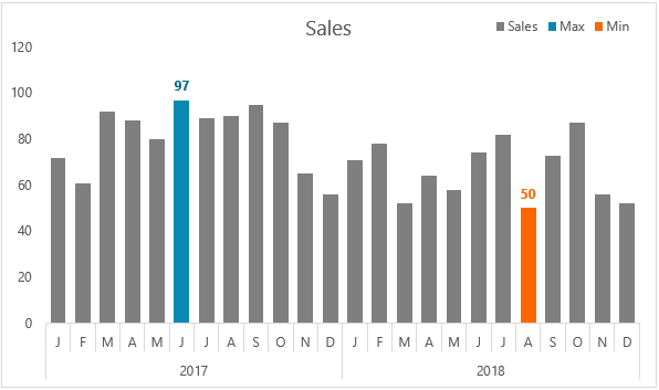
Change Column Colors / Show Percent Labels in Excel Column Chart

› Automate-Reports-in-ExcelHow to Automate Reports in Excel (with Pictures) - wikiHow Apr 13, 2020 · Excel will track every click, keystroke, and formatting option you enter and add them to the macro's list. For example, to select data and create a chart out of it, you would highlight your data, click Insert at the top of the Excel window, click a chart type, click the chart format that you want to use, and edit the chart as needed.

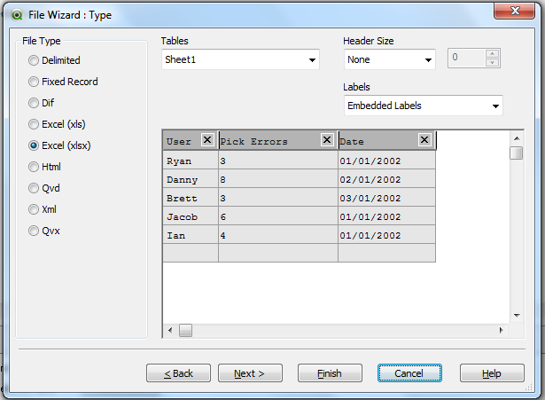
Solved: How to Display Excel sheet Column name - Qlik Community - 769330

Prevent Overlapping Data Labels in Excel Charts - Peltier Tech Overlapping Data Labels. Data labels are terribly tedious to apply to slope charts, since these labels have to be positioned to the left of the first point and to the right of the last point of each series. This means the labels have to be tediously selected one by one, even to apply "standard" alignments.

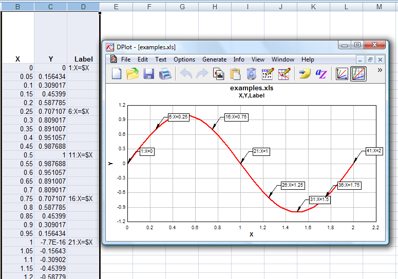
DPlot Windows software for Excel users to create presentation quality graphs

Use the Column Header to Retrieve Values from an Excel Table This post discusses ways to retrieve aggregated values from a table based on the column labels. Overview. Beginning with Excel 2007, we can store data in a table with the Insert > Table Ribbon command icon. If you haven't yet explored this incredible feature, please check out this CalCPA Magazine article Excel Rules.. Frequently, we need to retrieve values out of data tables for reporting or ...

How to add data labels from different column in an Excel chart?

Custom Data Labels with Colors and Symbols in Excel Charts - [How To] The way I know is to simply click the data label once and clicking it again will select the particular data label which you can then format with desired color. And of course you will have to do it for each data label separately. Tiring right? And above that it is "hard" coloring the labels.

31 How To Label Excel Columns - Labels Database 2020

peltiertech.com › text-labels-on-horizontal-axis-in-eText Labels on a Horizontal Bar Chart in Excel - Peltier Tech Dec 21, 2010 · In this tutorial I’ll show how to use a combination bar-column chart, in which the bars show the survey results and the columns provide the text labels for the horizontal axis. The steps are essentially the same in Excel 2007 and in Excel 2003. I’ll show the charts from Excel 2007, and the different dialogs for both where applicable.

stepping forward to learn excel daily..: Sub - Divided or Component Bar Diagram

How to Change Excel Chart Data Labels to Custom Values? You can change data labels and point them to different cells using this little trick. First add data labels to the chart (Layout Ribbon > Data Labels) Define the new data label values in a bunch of cells, like this: Now, click on any data label. This will select "all" data labels. Now click once again.

Label Columns In Excel - Ythoreccio

engineerexcel.com › 3-axis-graph-excel3 Axis Graph Excel Method: Add a Third Y-Axis - EngineerExcel However, in Excel 2013 and later, you can choose a range for the data labels. For this chart, that is the array of unscaled values that was created previously. So I right-clicked on the data labels, then chose “Format Data Labels”. Then, in the Format Data Labels Task Pane, I selected the box next to “Values from Cells”. This opens a ...

Business Diary: October 2011

How can I add data labels from a third column to a scatterplot? Do you want to add data labels to the 3rd column values in the chart? Highlight the 3rd column range in the chart. Click the chart, and then click the Chart Layout tab. Under Labels, click Data Labels, and then in the upper part of the list, click the data label type that you want.

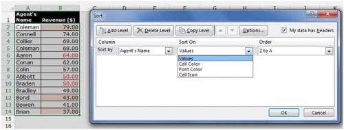
How to Sort data in Microsoft Excel

Excel, giving data labels to only the top/bottom X% values 1) Create a data set next to your original series column with only the values you want labels for (again, this can be formula driven to only select the top / bottom n values). See column D below. 2) Add this data series to the chart and show the data labels. 3) Set the line color to No Line, so that it does not appear! 4) Volia! See Below! Share

Ease the Pain of Data Entry with an Excel Forms Template | Pryor Learning Solutions

› excel-stacked-column-chartStacked Column Chart in Excel (examples) - EDUCBA Overlapping of data labels, in some cases, this is seen that the data labels overlap each other, and this will make the data to be difficult to interpret. Things to Remember A stacked column chart in Excel can only be prepared when we have more than 1 data that has to be represented in a bar chart.

How to Create Multi-Category Chart in Excel - Excel Board

How to Print Labels From Excel - EDUCBA Navigate towards the folder where the excel file is stored in the Select Data Source pop-up window. Select the file in which the labels are stored and click Open. A new pop up box named Confirm Data Source will appear. Click on OK to let the system know that you want to use the data source. Again a pop-up window named Select Table will appear.

How to Sort data in Microsoft Excel

How to create Custom Data Labels in Excel Charts To customize it, click on the arrow next to Data Labels and choose More Options … Unselect the Value option and select the Value from Cells option. Choose the third column (without the heading) as the range. Now we have exactly what we want. Some labels may overlap the chart elements and they have a transparent background by default.

Select data for a chart - Excel

How to Add Labels to Scatterplot Points in Excel - Statology Next, click anywhere on the chart until a green plus (+) sign appears in the top right corner. Then click Data Labels, then click More Options… In the Format Data Labels window that appears on the right of the screen, uncheck the box next to Y Value and check the box next to Value From Cells.

How to Create Multi-Category Chart in Excel - Excel Board

Using Data Labels from a Third Data Column in an Chart Excel 2013, allows you to select Data Labels locations from a Dialog box Prior to that it had to be done either manually or via a Macro To do it manually Select a Series Add a Data Label Select the Data Labels Then select an Individual Data Label In the formula bar =$D$2 (Cell reference to your new labels) Repeat for all Labels G guna_sekar87

Merging 2 spreadsheets on Excel 2010 - Super User

How to Create Mailing Labels in Word from an Excel List Step Two: Set Up Labels in Word. Open up a blank Word document. Next, head over to the "Mailings" tab and select "Start Mail Merge.". In the drop-down menu that appears, select "Labels.". The "Label Options" window will appear. Here, you can select your label brand and product number. Once finished, click "OK.".

Share :